Dear @Jason.Jonkman
Yes, this is the work I want to do in the future. But before that, I hope to generate a large number of dense grids. When the area is large (such as my current grid height of 180 and width of 380), it is difficult for me to generate high-precision grids. I want to know if this is related to the code or the hardware performance of the computer?
Also, I would like to know what aspects I need to pay attention to if I want to generate a non-uniform discrete grid at the bottom, or even a grid that varies over time (similar to the elevation distribution of waves)?
I’m not familiar enough with the TurbSim source code to provide guidance on modifications to support nonuniform grids. To get around this existing limitation of TurbSim, when using TurbSim to generate inflow for FAST.Farm, we typically recommend using Mod_AmbWind = 3, which makes use of multiple TurbSim files–one for the coarse, low resolution domain around the farm and separate ones for the high-resolution domains around each wind turbine. Guidance for using Mod_AmbWind = 3 is provided in the online FAST.Farm documentation (4.2.15.6. Modeling Guidance — OpenFAST v3.5.2 documentation) and Python scripts to automate the process are available in the OpenFAST Toolbox: openfast_toolbox/openfast_toolbox/fastfarm at main · OpenFAST/openfast_toolbox · GitHub.
Regardless, TurbSim is not parallalized, so, I would expect you’d have difficult if the number of grid points per plane exceeds about 1600 points. Here is a link to an older topic that discusses the CPU time expected with TurbSim simulations: TurbSim CPU Times
Sorry to reopen the discussion, but I have questions about ambient mode 3. I used the various scripts provided in this discussion and applied them to my case study involving two aligned 22MW turbines. After generating my synthetic wind with TurbSim and obtaining my three files Low.bts and High_T{i}.bts, I do not find the offset presented by @Regis.Thedin.
Hi Tom,
The offset is done automatically by the toolbox and takes into account the mean wind speed and the location of each individual turbine. The time series used for the constrained TurbSim execution of the high-res boxes contain that offset.
I’m not sure where exactly these curves you showed are coming from, but I suggest you plot 4 curves to help identify the problem: (i) time series from the low-res at the location of interest (say, T1); (ii) the time series as given by the text file given as input to the high-res box of the same location of interest; (iii) the time series at the center of the high-res box, as generated by TurbSim; (iv) the wind speed as observed by the turbine.
The curves (ii-iv) should all match (within interpolation tolerances), and should all the offset from curve (i).
Thank you for your response
I have plotted the four curves as requested. So, I plotted (i) the low.bts file at hub level. I plotted (ii) the time series extracted from the low.bts file at hub level. I plotted (iii) the data from the HighT1.bts file and finally the data from the FAST.Farm simulation (FAST.Farm.T1.out). I do get an offset, but it’s approximately 8 seconds. However, the first turbine is located 1000 meters from the leading edge. Normally, if I use the formula ‘round((xt/Vmid.mean())/bts.dt)’, I should be around 150 seconds of offset with xt = 1000, Vmid = 18, and bts.dt = 0.35.
I’m not sure why you are getting an offset of only 8 seconds. The offset is calculated on these lines. As you can see, the same equation you just gave is the one used to compute start_time_step. Can you put a breakpoint around those lines and double check what numbers you are seeing, in addition to a quick plot of uvel? I would also check what xt, Vmid and bts.dt are and if there is any inconsistency with what you were expecting.
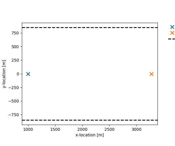
When I plot the setup using the plotSetup function, I obtain the figure above. Upon closer inspection, it seems that the TurbSim reference frame is near the first turbine. Could this explain the 8-second offset?
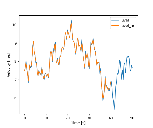
I have also plotted uvel and uvel-hr, which are defined in the code as follows:
The domain around the turbines is trimmed down. There is no need to have flow field much ahead of the most-upstream turbine or much further downstream the most-downstream turbine. The parameter extent* (e.g., here) gives an extra spacing around the farm. If you set such values to zero, you will have a domain very tight around the convex hull of your farm.
When you mentioned your turbine was at x=1000, I interpreted as 1000m from another upstream turbine. If your turbine is at x=1000, but there is nothing upstream of it, then for TurbSim (and FAST.Farm) purposes, this first 1000m of your domain do not matter. It makes sense that you are seeing a very short offset if your turbine is very close to the edge of the trimmed-down domain.
If you are using the toolbox for FAST.Farm case generation, you can also use <your_object>.plot() to see the overall layout and domain.
If your T2 is at x=3200 and your T1 offset is 8s, I would expect that the offset of your second turbine is around 350+8=358s.
Regarding your plot, can you clarify exactly which arrays you are plotting against which time arrays? It’s unclear why the orange curve is stopping at 40s.
Apologies for the delayed response—I’ve been working on another project in parallel. I’ve since investigated the issue in more detail.
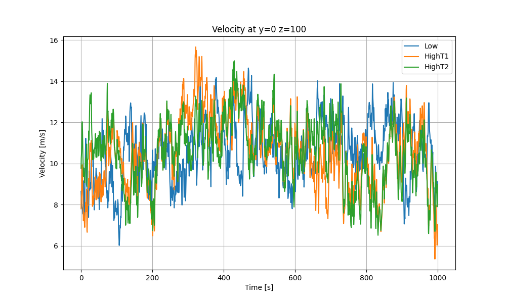
To verify the behavior, I used a simple test case with two turbines separated by 1000 meters, with a wind speed of 10 m/s. When comparing the velocity time series, I observed a shift between the uvel_roll and the velocity from Low.bts (uvel_brut), which is exactly 100 seconds, as expected.
However, when I extract the time series at hub height and generate the HighT1 and HighT2 parameters, the velocity extracted at hub height matches well with the TurbSimHighT1 data created from the extraction—the two curves are quite similar.
But when I run TurbSim, I notice a significant difference between the Low.bts and HighT{i}.bts files. The expected shift is no longer visible, even though I used the exact same RandSeed for all three files.
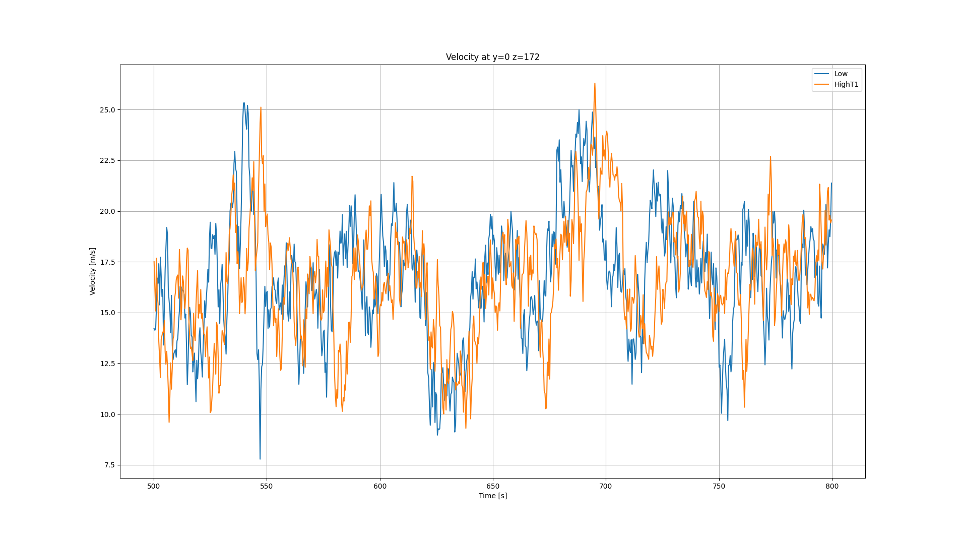
This leads me to wonder: Do I need to interpolate the data between the Low and High grid files to ensure the nodes align at hub height? When I interpolate the data from Low.bts to match the spatial discretization of the High file, the resulting wind values at index (iy, iz)=ts.closestPoint(y=0,z=172) are as follows:
Interpolated Low: Index (16, 17), Wind value: 8.171723991633412
Original Low: Index (8, 9), Wind value: 8.050255745435102
HighT1: Index (16, 17), Wind value: 8.233654525207282
HighT2: Index (16, 17), Wind value: 10.247062072996263
As you can see, there is a notable discrepancy between the interpolated Low data and the HighT{i} data.
There are no requirement that the a grid point of the low-resolution box is at the turbine location. In fact, it likely will not be. The high-resolution, on the other hand, is centered around the turbine. When we pull a time-series from a point in the low-res to drive (constrain) the high-res, we do so at the nearest point. Since that point may not be co-located with a point on the high-res, we add an offset. There is a long comment there explaining the process.
To help narrow down the issue, can you place your turbine at a grid point of the low-res? That way, all the velocity values should match. Also- if possible, please share the inputs you are giving to the FAST.Farm case generation code. As I mentioned above, I could not reproduce the issue, so a reproducible case would help greatly.
Thank you for your response. I understood the process and have successfully obtained realistic wind results using ambient mode 3, with matching time steps between the low- and high-resolution files.