I am currently using ACDC to linearize wind turbine generators and have encountered the following issues:
If I use ACDC for linearization, do I first calculate the steady-state rotational speed corresponding to each wind speed in the time domain, then substitute it into ACDC, and finally perform linearization using ACDC? If so, ACDC should automatically disable GenDoF. Is my understanding of ACDC linearization correct?
2. If I skip ACDC and linearize solely by fixing wind speed and enabling GenDoF, this approach seems equally convenient compared to my described ACDC method. Where exactly does ACDC offer advantages? Is it merely for easier Campbell diagram plotting and mode shape visualization? However, modifying Campbell diagrams isn’t particularly convenient within ACDC.
3. Currently, I wish to study the aeroelastic stability of wind turbine blades. I lack familiarity with the principles of linearizing BEM theory and beam models. Could you recommend relevant research papers for my study?
Many thanks beforehand,
regards,
ACDC can compute Campbell diagrams with or without aerodynamics. Either way, you need to specify what rotor speeds to linearize about. With aerodynamics enabled, for a given turbine, you would likely already know what the steady-state rotor speed is as a function of wind speed (this information is published if you are using one of the OpenFAST reference models, such as the NREL 5-MW baseline turbine or the IEA Wind 15-MW RWT). But if not, you can compute these separately from OpenFAST at different wind speeds before running ACDC. ACDC does not require that GenDOF be disabled, and if it is enabled, ACDC will use OpenFAST’s trim solution to figure out the appropriate generator torque (below rated) or blade-pitch angle (above rated) that will give the desired rotor speed at each wind speed at the steady-state condition.
ACDC automates the process of setting up the OpenFAST input files for each operating point, running OpenFAST to compute the steady state plus linearized solution, applying the multi-blade coordinate transformation (MBC3), plotting the Campbell diagram, and visualizing the mode shapes. You could certainly do some of these steps by hand, but it should be easier to use ACDC for all steps.
Here are few papers that describe the linearization capability available in OpenFAST:
Thank you very much for your explanation and the paper you provided. I apologize for the delayed response.
I still have the following questions:
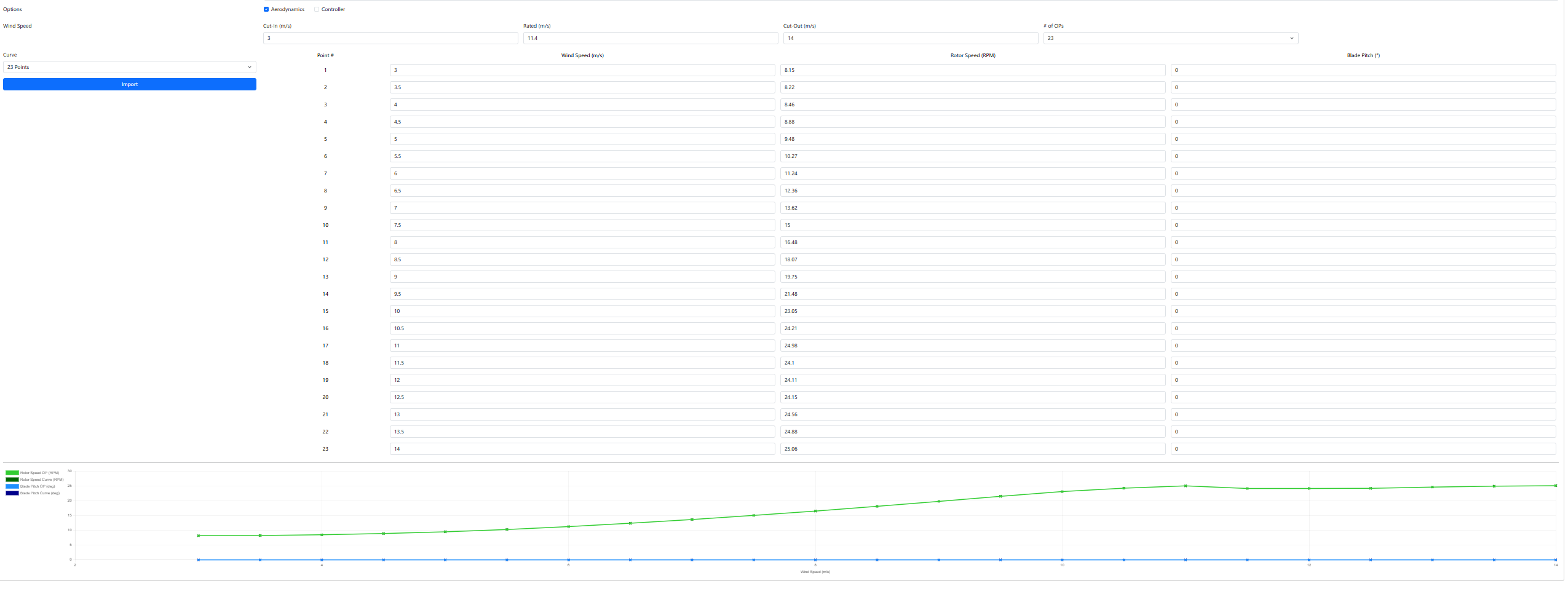
1. For a given wind turbine, there is indeed a steady-state relationship between rotor speed and wind speed. However, this should describe the relationship during normal operation. If I need to perform linearization for runaway or shutdown conditions, my understanding is that I should calculate the rotor speed reaching a stable value at different wind speeds with GenDOF enabled, then substitute these values into the ACDC operating point for linearization. I compared my approach with time-domain simulations under runaway conditions and found the flutter critical speed does not match. Below are my settings for wind speed and rotor speed in the time-domain simulation.
2. I am unsure whether my calculation of steady-state rotor speed under runaway conditions is correct. If my approach is valid, this workflow seems more complicated than the time-domain simulation.
3. I still struggle to grasp how OpenFAST linearizes the nonlinear equations of each module after identifying the operating point and combines them into a linear state-space model for the entire system. Could you briefly explain this to aid my understanding? Additionally, I remain uncertain whether a linearized version of BEM theory exists, as I’ve only encountered forms involving state equations and output equations.
4. What linearization methods exist for wind turbine stability analysis? I’m only familiar with adding a small disturbance followed by Taylor expansion. Are there other approaches?
5. Can the aeroelastic coupled equations be linearized?
Apologies for the lengthy list of questions. Thank you for your patience in reviewing them. I look forward to your response.
Regarding (1-2), I’m not sure I fully understand your questions. From your figure, it looks like you are simulating a runaway condition in the time-domain in OpenFAST. But how are you doing the equivalent in ACDC? For the linear model to be valid, the operating point must (OP) be in quasi-equilibrium state. I could certainly see using ACDC to compute OPs and linearizations for different mean wind speeds and different rotor speeds.
Regarding (3-5), OpenFAST uses a combination of analytical linearization and finite-differencing to compute the linearized system matrices (depending on the specific module) and these are combined together algebraically. One paper I should have linked to above is our original FAST modularization paper (https://docs.nrel.gov/docs/fy13osti/57228.pdf), which explains the overall approach OpenFAST uses to combine the linearized models from each module together (the paper I did link to above, 67545, builds upon 57228). The linearization of BEM within AeroDyn is done numerically via finite differencing. And, yes, OpenFAST can linearize the aero-elastic equations by combining the linearizations of the structural modules (ElastoDyn, BeamDyn) and the aerodynamics module (AeroDyn) together.
Thank you very much for your explanation and the paper you provided. I apologize for the delayed response.
How can I simulate this runaway operating condition using a linearized approach? Specifically, how do I determine the rotational speed corresponding to the wind speed at the respective operating point?
Well, a runaway condition is by definition not in a quasi-equilibrium state. So, the workaround I would suggest is to use ACDC to compute different OPs and linearizations for different mean wind speeds and different rotor speeds around the runaway condition. If you know what condition the runaway occurs in terms of wind speed and rotor speed from other time-domain simulations, I would use those as the target OP for linearization.
Do you mean I need to use uniform wind to simulate all operating points in the test case? For example, should I set a fixed wind speed of 3 m/s and take the average rotational speed from the last cycle? If I follow this approach, when the operating point intervals are very small—say, from 3 m/s to 25 m/s—there would be too many operating points. Wouldn’t the time-domain method become quite cumbersome?
Perhaps I’m not understanding. I was picturing you trying to capture a specific runaway condition. Are you trying to consider many runaway situations under different conditions?
I am currently examining specific loss-of-control scenarios, with the corresponding rotational speeds and wind speeds shown in the diagram above. I have obtained the Campbell diagram as illustrated below, but the stall rotational speed is approximately 19 rpm, which does not align with the time-domain result of 24 rpm. Therefore, I suspect there may be an issue with the wind speed and rotational speed at the operating point, as depicted in the figure below. How should I proceed to resolve this problem?
I’m not understanding the following comment in relation to the ACDC data you are shared; can you clarify what your concern is with the ACDC result and what your question is?
What I mean is that the results calculated in the time domain don’t match the rotational speed at zero damping ratio obtained from the Campbell diagram. I now suspect the issue lies with the operating point data, though I’m not certain. I hope you can help me resolve this problem so that the critical rotational speed in the Campbell diagram aligns with the results from the time-domain simulation.
Your time-domain solution involves a transient simulation that is not in equilibrium, so, I suspect that is one reason it does not match your results from ACDC, where an an equilibrium point (operating point) is being found.
If I understand correctly, you’d like to set the operating point equal to about 24.2 rpm at a wind speed around 10.5 rpm, but I don’t see that you’ve in your list of ACDC operating points.
Can ACDC validate the transient simulation results for unbalanced conditions in this time-domain scheme? If so, how should I set the operating point?
The time-domain simulation results indicate instability occurs at a rotational speed of 24.2 rpm and wind speed of 10.5 m/s. My ultimate goal is to use ACDC to verify the critical flutter speed obtained from the time-domain simulation. How would you proceed in this situation?
The model must be in quasi-steady equilibrium for the linearization to be reliably (otherwise, accelerations within the system will bias the stiffness matrix), which is why operating point determination is the first step in ACDC.
I would suggest executing ACDC for various operating points scattered around the runaway condition you want to analyze, e.g. wind speeds in the range of 10-11 m/s and rotor speeds in the range of 24-25 rpm (perhaps you want to widen these ranges a bit in case the quasi-steady state differs a bit from the transient state).
As per your instructions, I have set the wind speed range for the operating points to 8 to 11.8 m/s with 0.2 m/s increments, as shown in the figure below.
Furthermore, the resulting Campbell diagram still indicates a damping ratio of zero at approximately 8.5 m/s wind speed, which remains non-compliant with requirements, as shown in the figure below.
Can you clarify what TrimCase you are trying to use to compute a steady-state solution?
If your model is in unstable with negative damping, you’ll need to add damping to the model during the steady-state solution to ensure a steady-state solution can be found, i.e. nonzero Twr_Kdmp and/or Bld__Kdmp. These factors add damping to aid in calculating the steady-state solution, which is then removed before linearization.