Hi everyone,
I have encountered some difficulties regarding the linearization at region 2.
I am using OpenFAST in its latest version 3.1. and I am conducting a series of linearization of the NREL 5MW wind turbine. The following considerations have been taken:
- Operating points considered: 3:1:11 (wind velocities at region 1.5, 2 and 2.5)
- Modules activated: ElastoDyn, ServoDyn, InflowWind and AeroDyn v15
- TrimCase = 2: Internal torque controller recommended for region 2
- CalcSteady = True: In order to enable an automatic stationary state identification
- TrimTol = 0.001
- TrimGain = 1000
- VSCntrl = 1: As it is recommended in FASTv7 manual to conduct linearization
- VS_RtGnSp = 9999.9E-9
- VS_RtTq = 43093.55
- VS_Rgn2K = 9999.9E-9
- VS_SlPc = 9999.9E-9
After the linearization, we extracted the state matrices using fx_getMats.m Matlab’s function and analyze the temporary signals, as well as the stationary values of the parameters.
When analyzing the outputs at a 7 m/s linearization, we found that the parameter GenPwr did not correspond to the expected one at that velocity. Apparently, when the Generator-Torque controller is activated (VSCntrl=1), it seems that GenPwr is being calculated using the VS_RtTq nominal torque.
After linearizing the model at operating points between 3 and 11 m/s and analyzing the steady outputs of the system, we were expecting to obtain a pattern such as the red signal on the right (GenSpeed·GenTq). However, values of GenPwr did not match our expectations.
Is there something wrong in our input files (attached) or did somebody find a similar problem in its simulations?
On another note, has the LIDAR module already been added to OpenFASTv3?
Thank you in advanced.
Input Files
1 Like
Dear @Daniel.Aldaz,
Just a couple comments:
- The FAST v7 User’s Guide only recommends setting constant torque for
TrimCase = 3 (linearization of blade pitch in Region 3). For TrimCase = 2 (linearization of generator torque in Region 2 with fixed blade pitch), the generator torque is assumed to be calculated via the trim controller rather than with an internal torque controller in ServoDyn. So, effectively, you want ServoDyn to return zero torque. This can be achieved by setting in ServoDyn GenTiStr = True and TimGenOn > TMax, where TMax is the maximum simulation time set in the OpenFAST primary (.fst) input file.
- While the trim controller will calculate the generator torque needed to reach a steady-state solution, it is not tracking generator power. So, the ServoDyn output GenPwr will be calculated using the internally selected generator model (GenPwr = 0 when
GenTiStr = True and TimGenOn > TMax) regardless of the actual generator torque set by the trim controller. So, I wouldn’t rely on ServoDyn output GenPwr being accurate when enabling a trim solution.
I’m aware of the LiDAR module being implemented in OpenFAST, but the pull request has not been issued yet.
Best regards,
Dear @Jason.Jonkman,
First of all, thank you for your fast response.
I have been checking all the comments you made and considering its effect in the linearizations we are running. I followed your recommendation regarding the trim controller of region 2 linearizations, and I will probably consider HSShftPwr as a more reliable output of the Generator Power when enabling the trim solution.
Given that, we have found some unsual behaviors when studying the bode diagrams of the different outputs.
-
The low frequencies of the bode representation between the wind speed and the generator speed show an abnormal peak behaviour, which reminded us to the bode diagram of a closed loop simulation.
Besides, if we compare it with the same bode representation of a linear model obtained with FASTv7, the results were quite different for the lower frequencies.
-
On the other hand, when computing the bode between the wind speed input and the blade pitch, we were not expecting to obtain any result at all. FASTv7 solution did give us an empty output between these two variables.
Even though it is very subtle (around -220dB), it makes us think that the linearization is being computed for a closed loop system of the wind turbine and not for the open loop itself (as this problem appears for all of the operating points considered in the linearizations).
We would be pleased if you could take a look to both problems and tell us what you think about them.
I attach the linear model (.mat) for all of the wind speeds considered as well as the input files (.fst and .dat) of the linearizations. Files
Thank you so much in advanced and best regards,
Dear @Daniel.Aldaz,
I don’t have much experience reviewing Bode diagrams, so, I can’t comment much on those.
Looking briefly at your OpenFAST model, I see that you have specified constant torque in ServoDyn, which is what we recommend using with TrimCase = 3. But for TrimCase = 2, I had recommended setting TimGenOn > TMax, which I don’t see set.
I only see that you are linearizing twice (NLinTimes = 2). Are you applying MBC3 and azimuth averaging over 2 azimuths? I would recommend increasing this to 36 linearizations (every 10 degrees of azimuth).
Also, I’m not sure how to interpret your MATLAB data. It appears that you have computed the linearized system for 23 different wind speeds; is that correct? Unfortunately, the MATLAB data structure doesn’t seem to store the state matrices, so, I can’t review those.
Best regards,
Dear @Jason.Jonkman,
Sorry for the misunderstanding. I forgot to update the new files (.fst and .dat) into the Google Drive, even though I had already followed your recommendations and used them in my current linearizations.
I have also increased the number of linearizations to 36 in order to consider a greater number of azimuths when applying MBC3. However the bode diagrams seemed to show the same trend as stated before.
I was computing a linearization for every wind speed in the 3:25 range.
In order to make it clearer, I have changed the MATLAB data of the Google Drive with the results obtained from the matlab function fx_mbc3 (MBC3). It contains two files with the linearizations at 9m/s and 12m/s (while NLinTimes = 36). Besides, the input files can also be found there.
Could you take a look at it? Thank you so much for all your help.
Best regards,
Dear @Daniel.Aldaz,
Well, I’ve reviewed your files a bit, and don’t see any obvious issues. I’m not sure what to comment on. Can you clarify your question?
Best regards,
Dear @Jason.Jonkman,
First of all, I am sorry for the late reply. I have been taking a close look at the linearization process conducted with OpenFAST v3.1.
My issue is related with the linear models obtained from the .lin after linearizing the system.
For example, in this case I will focus on Region 3 and compute a linearization with the following characteristics:
- Operating point: 16 (wind velocity at region 3)
- Modules activated: ElastoDyn, ServoDyn, InflowWind and AeroDyn v15
-
TrimCase = 3: Internal pitch controller recommended for region 3
-
CalcSteady = True: In order to enable an automatic stationary state identification
-
TrimTol = 0.001
-
TrimGain = 0.0045
-
TimGenOn = 0
-
VSCntrl = 1: As, in these cases, it is recommended in FASTv7 manual
-
VS_RtGnSp = 9999.9E-9
-
VS_RtTq = 43093.55
-
VS_Rgn2K = 9999.9E-9
-
VS_SlPc = 9999.9E-9
-
NLinTimes = 2: In this case I just want to analyze one azimuth to show my issue
After this process, the output file can be found in the following GoogleDrive, as well as the inputs files used for the linearizations.
Even though VSCntrl = 1 imposses a constant Torque Controller, when analyzing the system between ED Generator torque, Nm and SrvD GenTq, (kN-m) we were expecting to obtain a constant value of 0.001 (because of the change of units). However, the value of the D matrix, associated to these input-output, was completely empty.
This empty bode diagram makes us think that there is no direct relation between the input torque demand and the outputs of ServoDyn, such as GenTq and GenPwr (as a similar concept happens with the system and bode diagram between ED Generator torque, Nm and SrvD GenPwr, (kW)).
It seems that D’s state matrix has a complete empty row associated with those two outputs and I can not understand why. Besides, by comparing the results with an analogous linearization computed by FASTv7 software, we checked that only D matrix differed that much, as A, B and C matrices had very similar results for these input-output systems.
Are we missing some kind of DLL used by the Internal Torque Controller (of VSCntrl = 1) or is there something wrong in the extraction of D matrices done by the tool?
On another note, when I want to compute a single linearization (NLinTimes = 1) and CalcSteady = True, the linearization is conducted at the first time step. Is this done on purpose?
Thank you so much in advanced again for all your help.
Best regards,
Dear @Daniel.Aldaz,
Regarding the linear state-space input ED Generator Torque, Nm, I think the confusion arises because of how this input is defined. Linear state-space input ED Generator Torque, Nm represents a perturbation to the generator torque input to ElastoDyn. Normally within OpenFAST, the generator torque is calculated and output from ServoDyn and used as input to ElastoDyn. But in the linear model, the perturbation is performed only on the ElastoDyn input, independent from ServoDyn or the ServoDyn outputs. So, it makes sense to me that the rows associated the ServoDyn outputs SrvD GenTq, (kN-m) and SrvD GenPwr, (kW) in the D matrix are zero.
Regarding your last question, when CalcSteady = True, I would only expect OpenFAST to linearize at time zero if the time-domain solution is already in steady state, at least within the tolerance set (TrimTol).
Best regards,
Dear @Jason.Jonkman,
Thank you for your answer, that makes a lot of sense.
I did not perceive the changes that modularity introduced in the linearizations.
Having that in mind, which input-output signals of the other modules would you recommend to obtain a system between the torque demand and the generator torque/power output (similar to GenTq or GenPwr from ServoDyn).
Best regards,
Dear @Daniel.Aldaz,
I’m not sure I understand what you mean when you ask abut going from generator torque input and generator torque output. Wouldn’t these be one-to-one? Or perhaps you want to look at the influence of the generator torque input on the high-speed shaft torque output (ElastoDyn output HSShftTq). Likewise, perhaps you want to look at the influence of the generator torque input on the high-speed shaft power output (ElastoDyn output HSShftPwr).
Best regards,
Dear @Jason.Jonkman,
Yes, I wanted to analyze the influence of the linear state-space input ED Generator Torque, Nm on the generator torque and power outputs. It is a one-to-one relation but it could be helpful to check that it was working properly. I guess the only way will be to study the influence of the ED Generator Torque, (N·m) on the outputs of ElastoDyn you metioned (HSShftTq and HSShftPwr).
What would you suggest in order to represent a generator model so that we could transform ED HSShftTq, (kN·m) into a signal similar to the electrical SD GenTq, (kN·m)?

Besides, in simulation we designed a feedback loop controller entering the SFunc through the Generator torque (N·m) input (electrical generator torque to ServoDyn).
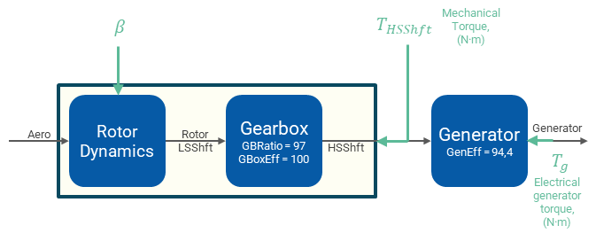
However, due to the modularity of OpenFAST, the only available torque input in the linear model right now is the ED Generator Torque, (N·m). I was wondering if this input corresponds to a mechanical or an electrical torque so that we can use the same controller structure or we will need to change it. In the figure shown below, does ED Generator Torque, (N·m) represents T_HSShft of T_g?
Thank you so much for all your answers, they are being extremely helpful in order to progress with our linearizations.
Best regards,
Dear @Daniel.Aldaz,
The input to the linear model, ED Generator Torque, represents a perturbation to the electrical generator torque (T_g). Basically, the generator torque operating point is the electrical generator torque commanded by Simulink, and linear input ED Generator Torque represents the perturbation of this torque. It is just that it linear input ED Generator Torque does not directly transfer in/out of ServoDyn.
Best regards,
Dear @Jason.Jonkman,
I’ve encountered some difficulties with the linearization in Region 2. I’ve gone through various discussions on this topic in forums, but I’m still uncertain about the issue. For calculating the steady responses, I’ve used the following settings: CalcSteady = True, TrimCase = 2, VSContrl = 0, GenModel = 1, and TimGenOn = 9999.9. Under a 4 m/s wind speed, the desired azimuth-averaged rotor speed is 7.18 rpm (as set in RotSpeed in ElastoDyn). However, after linearization with OpenFAST, the RotSpeed comes out as 10.43 rpm, which is significantly higher than the desired value. I’m not sure what is causing this discrepancy in my analysis. Could you please assist me in identifying the issue? I’ve attached the .fst, ElastoDyn, and ServoDyn files I used for reference.
Thank you in advanced
Xiaogang Huang
Dear @Xiaogang.Huang,
My guess is that your OpenFAST model is not actually reaching a steady-state solution; rather, the 10.43 rpm is simply the rotor speed reached at TMax = 350 s. Your model is not reaching a steady-state solution quickly because your TrimGain is too low. For TrimCase = 2 (generator torque), TrimGain should have the units of Nm/(rad/s) and a value of 0.001 Nm/(rad/s) is very low given that the expected generator torque for NREL 5-MW baseline wind turbine at 4 m/s is 2580 Nm. I would increase TrimGain from 0.001 to, say, 1/10th of rated torque (43094 Nm), so, around 4000 Nm/(rad/s) for your case. Does that solve your issue?
Best regards,
Dear @Jason.Jonkman,
Thank you very much for your quick response. Your suggestion was correct. I now have another question regarding how to sort the modal frequencies from MBC3. I know you provided an Excel file named “CampbellDiagram” for this purpose, but I would like to implement this in a MATLAB script. Could you please provide some guidance on how this can be done?
Best regards,
Xiaogang Huang
Dear @Xiaogang.Huang,
The MBC3 and Campbell Diagram scripts in the MATLAB Toolbox no longer need the old CampbellDiagram.xls spreadsheet, as all of the data needed are generated and handled by the scripts, as documented in the ReadMe here: GitHub - OpenFAST/matlab-toolbox: Collection of Matlab tools developed for use with OpenFAST.
That said, a much more user-friendly way of generating Campbell Diagrams and visualizing full-system mode shapes with OpenFAST has been developed and released through the Automated Campbell Diagram Capabilities (ACDC) application: GitHub - OpenFAST/acdc: ACDC: Automated Campbell Diagram Code. I would suggest using ACDC instead of the MATLAB scripts.
Best regards,
Dear @Jason.Jonkman,
I have attempted to run the provided MATLAB Toolbox to generate the sorted modal frequencies. However, I still have some questions regarding the sorting method. For example, I noticed that the code can identify multiple modes with the maximum value in a single state. However, I’m unsure why the code always selects the mode with the smallest magnitude for the identified frequency.
Best regards,
Xiaogang Huang
Dear @Xiaogang.Huang,
I’m not sure I understand what you are asking? Can you clarify or explain via an example?
Best regards,
Dear @Jason.Jonkman,
I found a .m file named “postproLin_OneLinFile” in the MATLAB Toolbox, which seems to be a basic program intended for beginners. It computes the sorted modal frequencies for a single linearization file. Attached are the output results displayed on the screen after running this code. In the “Mode_content” row, I noticed that multiple states may have the maximum magnitudes for a single mode, or in some cases, no state has the maximum magnitude for that mode (i.e. labelled as ‘NoMax -’ in the end). In these situations, how can we determine to which mode the frequency belongs?
Best regards,
Xiaogang Huang
Dear @Xiaogang.Huang,
Interpreting the results of an eigenanalysis takes some experience, such as knowing that tower-bending modes come in pairs (fore-aft, side-side), flapwise bending modes come in triplets (collective, asymmetric progressive, asymmetric regressive), etc. It also useful to visualize the modes to aid in their interpretation, which is one thing ACDC does so well, which I’d recommend using over the older MATLAB scripts.
Best regards,


