WISDEM tower/monopile optimization: effect of different initial configurations on optimal solution

[Henny.Bottini]

Hello everybody,

I am optimizing the tower/monopile of a 20-MW offshore wind turbine with the following settings:
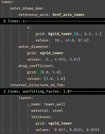
design variables: outer_diameter, layer_thickness (for both tower and monopile)
objective function: structural_mass
tower constraints: stress, global_buckling, shell_buckling, taper, slope, frequency_1 (lower_bound=0.05, upper_bound=0.3), thickness_slope
monopile constraints: stress, global_buckling, shell_buckling, taper, slope, frequency_1 (lower_bound=0.05, upper_bound=0.16), thickness_slope, pile_depth, tower_diameter_coupling
solver: SLSQP
To explore the design space, I run three optimizations with the above settings but different initial configurations (that is, different initial distributions of outer diameters and layer thickness):
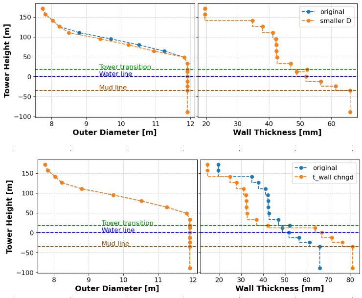
run 1: original configuration (plot label= original)
run 2: tower diameter reduced by 0.3 m at four points; layer thickness distribution original (plot label= smaller D)
run 3: wall thickness reduced by 10 mm all along the tower and increased by 15 mm all along the monopile; tower and monopile diameter distributions original (plot label = t_wall chngd)
See the plots below.

The three optimizations are successful. I can also verify that the constraints are respected by looking at these plots of the utilization factors for the von Mises stress, shell buckling, and global buckling (run 1: cyan, run 2: orange, run 3: green):

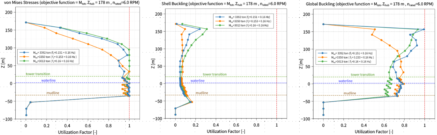
and the values of the 1st natural frequency of the monopile optimal designs are:
run 1: 0.151 Hz < 0.16 Hz
run 2: 0.153 Hz < 0.16 Hz
run 3: 0.16 Hz = 0.16 Hz
Summing up the values of tower mass and monopile mass found in the output file, the total structure masses are:
run 1: 3392 ton
run 2: 3350 ton
run 3: 3013 ton
So there is a difference in total mass values of about -1% between run 2 and run 1, and a difference of about -10% between run 3 and run 1.
The distributions of outer diameter and wall thickness of the optimal designs also change:

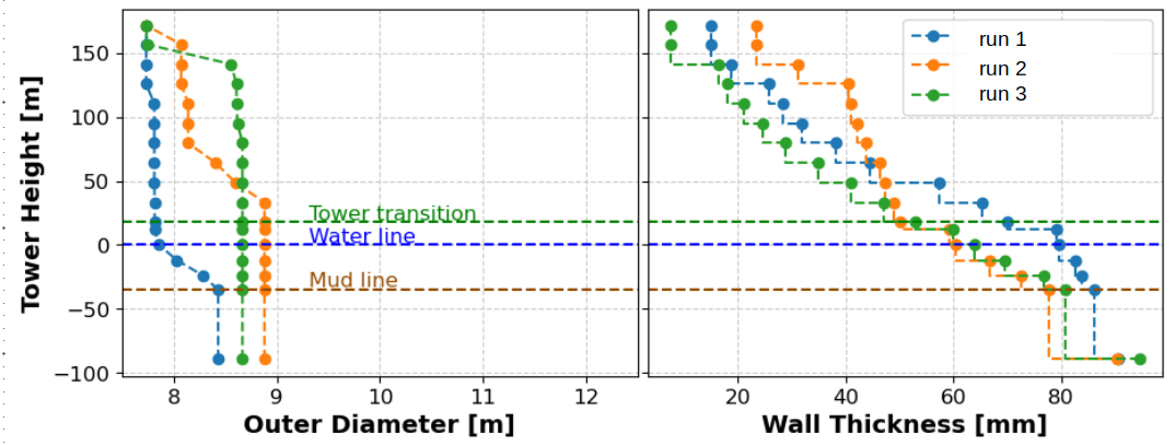
the diameter distributions differ of as much as about +1 m between run 2 and run 1 and between run 3 and run 1; the thickness distributions differ of as much as ~20 mm between run 2 and run 1 and between run 3 and run 1.

Now I am puzzled by the following questions:

1. I think that the difference in structural mass of about -1% between run 2 and run 1 is negligible, so I might consider those two optimizations to have output the same minimum for the structural mass. If so, why the diameter and thickness distributions of the optimal designs are not practically the same? If not so, can actually a difference of -0.3 m in the diameter at four points of the initial configuration of only the tower make a difference of as much as ~1 m along the optimal configuration of the tower and the monopile?

2. Can a difference in only the thickness of the initial configuration be responsible of differences in the outer diameter distributions of the optimal design?

3. Finally, how can the objective function structural mass for this relatively simple (correct me if I am wrong) optimization problem turn out to be multimodal, that is, to have different local minima instead of a single minimum?

I would really appreciate if someone could help me understand these results.

Thank you for your time and attention

[Garrett.Barter]

These are classic questions for optimization practitioners and often arise as one moves from theory to practice. Gradient-based optimization is heuristic, meaning it is path dependent and the path will change depending on initial conditions, algorithm settings, and convergence tolerance. With so many constraints, the regions of validity in the design space are not contiguous, so you are likely to find local minima. Additionally, with finite differences supplying the gradients, the gradients will be noisy and the algorithm won’t always proceed along the ideal path. Maybe you could overcome this by setting convergence tolerances that are tiny (~1e-10 or less), but then you would be waiting forever for convergence. These are all standard optimization issues and in no way unique to WISDEM or wind problems.

With all these challenges, a common practice in global optimization to improve rigor is “multistart” (which you can Google- apparently there is even a Matlab function for it). You essentially give many different initial conditions or settings, sometimes even dozens or hundreds of different ones, and either look for the best overall solution or look at trends among the results.

[Henny.Bottini]

Thank you very much Garrett for your (always) fast reply.
I’ll keep varying the initial configuration of the tower and monopile some more times to have more optimal design to compare.
Best,
Henny

[Henny.Bottini]

I have tried the multistart approach you suggested by running thirty times the WISDEM example case 05_tower_monopile/monopile_driver.py. I chose it over my current optimization problems because it finishes very much more quickly.

For each optimization I slightly changed the initial configuration of the tower and monopile at some points (manually in the nrel5mw_monopile.yaml file); for each optimization there is only one change at one point; the changes consisted in increasing or decreasing the diameter of some percent of the original value (see the figure below).

Twenty nine optimizations succeeded (I mean, WISDEM output was Optimization terminated successfully…Optimization Complete) and one crashed.

I plotted the optimal values of structural mass (the objective function of the optimization) to look for patterns, and the result is the figure below.

Seventeen of the twenty nine structural-mass values cluster in the range 600~650 ton, seven are between 750 and 900 ton, three around 700 ton, and there are two extreme values, with the value for the heaviest optimal design far away from all the others. Eight of the twenty nine values in the 600~650-ton range are actually coincident (structural mass = 630 ton), and the corresponding optimal designs are identical.

Then, I checked the optimization constraints, that is the distributions along the tower/monopile of the von Mises utilization factor, the shell buckling utilization factor, the global buckling utilization factor, and the value of the monopile 1st natural frequency. The plots below are representative of most of the utilization factors’ trends.

The constraint on global buckling is active at just one point, and is the only constraint active; in four of the twenty nine results the constraint on 1st natural frequency is the only one active; and eleven results have no constraint active at all. Now I am wondering:

1. The clusters in the distribution of the structural-mass values are the trends you mentioned in your answer just above: am I right?
2. If the optimizer is looking for the lightest structure possible and the optimization is successful, shouldn’t the optimal design show at least one utilization factor at 1.0 or close to 1.0 along most of the tower/monopile height (like in my plots at the beginning of this post)?
3. How should I judge the optimal designs that have no constraint active? Why, actually, they have no constraint active? It’s the first time that I see this kind of result…

Thank you Garret

[Henny.Bottini]

regarding the point 3 in the above post, I was wrong. It is not true that some cases have no constraint active. The example
runs the optimization for two design load-cases, and I was checking the utilization factors only for one of them. Checking also the other results, I can see that there is always one point where the utilization factor is 1.0. But again only one or two points along the tower and monopile, so I am still puzzled as written at point 2 of the previous post.

Now, I 'd like to have another point clarified.
I use compare_designs to compare the optimal configuration to the initial configuration. So I give as inputs the corresponding .yaml files, on the command line I read Running WISDEM for the initial configuration and loading WISDEM data for the optimal configuration, and the plots are generated:

Here I show the results from the original WISDEM example case that is run by monopile_driver.py. It happens that the optimal design coincides with the initial design. But, my point is that the plotted values of tower wall thickness of the initial configuration are not the same as in the nrel5mw_monopile.yaml file:

The tower top wall thickness in the plot is not 19 mm, but 22 mm (the second value of the array and not the first one).
The tower outer diameter values in the plot are the same except for the bottom point, and all the values for the monopile plots are the same as in nrel5mw_monopile.yaml file.
Why there is this difference in the tower top wall thickness? I read in the header of compare_designs.py “This script runs an instance of WISDEM for each yaml file”: what does exactly that mean? A single optimization step (so that design variables can get changed a bit)?
I find this difference also when I run an analysis instead of an optimization. That is, I prepare a geometry input file, and run WISDEM
with the analysis option driver/optimization/flag set to False, then I run compare_designs on the analysis output file to see the trends of outer diameter and wall thickness, and the wall thickness plotted differs from that in the geometry input file.

Thank you for your time and attention